mlsn-nitrogen-rate-kikuyu

MLSN has never included a soil-test nitrogen guideline, because available soil nitrogen tests do not reliably predict nitrogen supply for intensively managed turf. Nitrogen recommendations are developed separately, from expected growth or clipping production. That one fact explains most of the trouble that follows when the method gets carried off golf greens and onto sportsfields.

As an example, suppose a kikuyu (Pennisetum clandestinum, syn. Cenchrus clandestinus) sportsfield in Sydney, under regular winter football traffic, is supplied with 100 kg N/ha per year. The soil tests come back above the MLSN guidelines for potassium and phosphorus, the calculation returns no requirement, and the programme looks fine on paper. Then the field wears and becomes thin through the central corridor and doesn’t recover.

That is a hypothetical, and a real failure like it would need traffic load, drainage, compaction, irrigation and recovery time investigated before anyone blamed the nitrogen. But whatever the cause turns out to be, it isn’t an MLSN failure. Too often the soil test method gets the blame for a nitrogen decision it played no part in.

MLSN’s developers have consistently said it doesn’t set nitrogen rates, and Woods has said so in print for years. What I keep seeing is the post-mortem: a programme fails on a worn field, and the soil test method carries the blame because its name was on the paperwork.

What MLSN covers, and what it doesn’t

Woods, Stowell and Gelernter built MLSN from a database of soil tests taken under turf that was performing well at the time of sampling. They collected 16,163 Mehlich 3 results (Mehlich 3 is one of several lab methods for extracting nutrients from soil), kept the 3,683 from soils with a low capacity to hold nutrients and a pH between 5.5 and 8.5, and fitted a curve to the spread of values for each element.

The guideline is set where only 10% of those good-turf samples fall lower. In other words, nine out of ten soils under good turf held more than this. The current guidelines, as published in Woods’s MLSN cheat sheet and the PACE Turf table, are, in ppm Mehlich 3: K 37, P 21, Ca 331, Mg 47, S 6. The calcium and sulphur figures have both been revised down since the 2016 preprint, which gave 348 and 7.

Nitrogen isn’t on that list, because soil tests don’t predict N supply usefully in turf. Woods says plainly that N comes from a growth potential estimate or from measured clipping yield, worked out separately.

So when a programme described as “MLSN-based” carries a nitrogen rate, that rate came from somewhere else, usually growth potential and sometimes habit.

One caveat on scope. The derivation is a 2016 PeerJ preprint rather than a peer-reviewed paper, and Woods put the underlying data in the public domain and invited others to use it.

I have not found published work testing how well the guidelines predict fertiliser requirements on heavily trafficked kikuyu sportsfields, where turf must recover quickly and roots may be restricted by compaction. That is a separate question from whether the nitrogen assumptions that sit alongside MLSN hold on those surfaces, and I haven’t found published work on that either.

Neither gap means the guidelines are wrong there. It means their performance under those conditions hasn’t been established in anything I have found.

How GP can produce a 100 kg nitrogen budget

Run the PACE Turf growth potential model for Sydney and the number stops looking arbitrary.

Growth potential (GP) converts the average monthly air temperature into a score between 0 and 1. A score of 1 means the temperature is at the grass’s optimum, and the score falls away the further the temperature moves from it. Two numbers set the curve: the optimum temperature, written to, and a width term, written var, which controls how fast the score drops as you move away from the optimum.

The equation is GP = exp(−0.5 × ((t − to) / var)²), where t is the mean monthly air temperature. For warm-season (C4) grasses in Celsius, to is 31°C and var is 7.

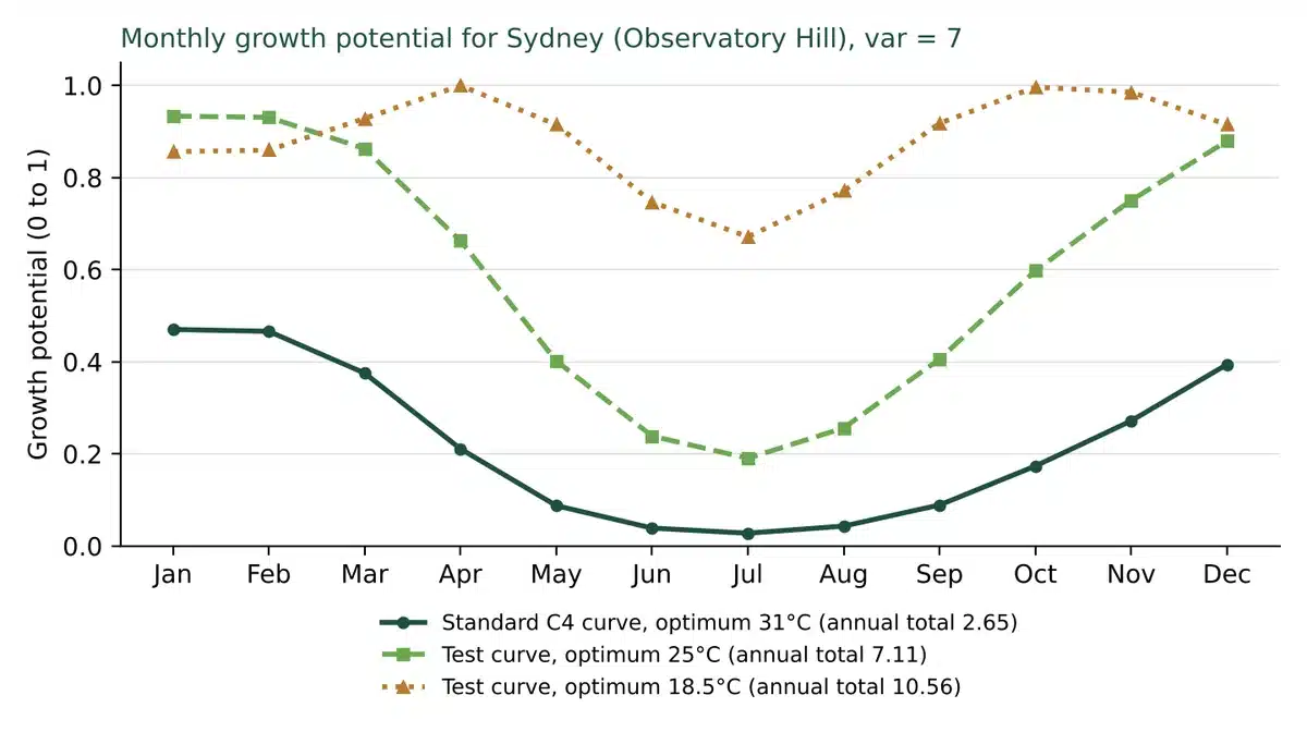
Using the Bureau of Meteorology all-years record for Observatory Hill (site 066062) and taking each month’s mean as the average of its mean maximum and minimum, Sydney’s monthly means run from 12.3°C in July to 22.4°C in January. That gives a monthly GP series peaking at 0.47 in January and adding up to 2.65 across the twelve months. The full monthly inputs and results are in the appendix. For comparison, a grass sitting at its optimum all year would score 12.

Distribute 100 kg N/ha in proportion to monthly growth potential and January, the peak month, receives about 18 kg N/ha. That is 1.8 g N/m², modest even for a warm-season golf green in midsummer.

An index is not a dose

GP does not set a nitrogen rate by itself. It produces a score, and the nitrogen rate depends entirely on how somebody converts that score into kilograms. That conversion is where most of the trouble starts.

Nor is GP a good predictor of how fast grass actually grows from week to week. Zhou and Soldat (2021) tested it against 2,190 clipping collections on a Wisconsin bentgrass green, and it explained about 1% of the variation in clipping yield. It was never built for that. It is built for spreading a season’s nitrogen across the months.

The case for leaving the equation alone

There is a good argument against changing the GP equation at all, and it comes from Woods himself. He has written that he no longer recommends adjusting it, and the reason is comparability.

A GP of 1 is not literally how grass grows. It is a number, and its usefulness is that it can be compared: two sites on opposite sides of the world can report something like organic matter accumulation against a GP for the year and the comparison means something, but only while everyone runs the same equation. That comparability applies to the calculated index, not necessarily to actual growth rates between species.

Start customising and your GP becomes unique to you, informative locally and meaningless for comparison with other sites. His advice is that if you will never compare your site to another, adjust away, but once comparisons are being made, go back to the standard form.

I agree with that objection, and it points to the fix. If GP is an index rather than a growth prediction, then what has to change for kikuyu is the kilograms of nitrogen you assign per unit of GP.

Where the kilograms come from

Woods’s own published conversion multiplies each month’s GP by a monthly maximum nitrogen rate: 4 g N/m² (40 kg/ha) for couch (bermudagrass in his text), 3 g for Poa annua and 2 g for bentgrass. He says those figures are based on the rates turf managers use to produce good turf, and he recommends measuring clipping volume to adjust them.

Keep the standard equation and a Sydney kikuyu field returns an annual GP sum of 2.65, which is perfectly serviceable as an index. But the nitrogen rate attached to it comes from golf turf, on different species, under a different loss pathway. There is no reason it transfers. Either you change the constant or you change the conversion, and a different conversion may be justified for kikuyu even if you keep the standard constants. What you cannot do is carry both across unexamined.

Clipping management is another reason the conversion may not transfer, and it points to less nitrogen, where traffic points to more. Golf greens, where those rates come from, normally have clippings removed. Most sportsfields return them.

In a two-site Connecticut study on a cool-season lawn mix, Kopp and Guillard (2002) found that returning clippings raised nitrogen recovery severalfold and allowed nitrogen to be cut by half or more with no loss of quality. At one site, no nitrogen with clippings returned matched 392 kg N/ha with clippings removed. That was a cool-season lawn, not kikuyu, but the principle applies: a borrowed golf rate can be too high on one count and too low on another, which is why it needs checking against measured growth.

The model is fine; the failure is reading an index as a dose.

The constant nobody looks at belongs to no species in particular

The published constants come in two sets: one for cool-season grasses such as ryegrass, fescue and bentgrass, which botanists call C3, and one for warm-season grasses such as couch and kikuyu, called C4 after the way they fix carbon. The C4 optimum of 31°C is a single warm-season value. It isn’t assigned to couch, kikuyu, zoysia or any other species, and the standard model offers no species-level alternative.

The available kikuyu temperature literature suggests an optimum below the generic C4 value of 31°C, although it does not establish the value the GP equation needs. Pinning down how much lower is harder than it should be.

Russell and Webb (1976) give 18 to 30°C, which is a growth range and not an optimum. Cook et al. (2005) give optimal average day temperatures of 16 to 21°C, which is a different quantity again: the GP equation takes mean monthly air temperature, and mean daily air temperature is not the same thing as mean day temperature. I have not read either original.

Russell and Webb are quoted in a review paper on kikuyu by Muscolo and colleagues, and the Cook figures come from Feedipedia, an online feed database run by the FAO and French agricultural research agencies. Treat both as indicative rather than as values you can put into the model.

The only measured kikuyu temperature response I have found is from Northland pasture, where Goold (1979) found winter growth rose by about 3.4 kg of dry matter per hectare per day for each degree of grass minimum temperature. That shows kikuyu growth tracking temperature closely in the cool months, but it is pasture data and does not give an optimum either.

Testing a lower optimum

Woods himself suggested an optimum of about 25°C for kikuyu (and 18°C for Poa annua) in a 2013 technical paper, as an adjustment rather than a value fitted to growth data, and before his later advice against adjusting the equation at all. It also sits close to the midpoint of the two published optima, C3 at 20°C and C4 at 31°C (25.5).

To test how much the answer depends on that one number, I have rerun the model at 25°C. Read it as a test value for a C4 grass whose optimum sits below the generic one, not as a fitted parameter. The point of the exercise is to show how sensitive the nitrogen figure is to the constant, not to claim kikuyu needs a particular amount more nitrogen.

What the change does to nitrogen

Substituting 25°C and changing nothing else moves Sydney’s warmest month from nine degrees below the optimum to two and a half below it. What that does to the nitrogen figure depends on how a programme turns GP into kilograms. The table compares three methods. Method B is Woods’s published approach, using his couch (bermudagrass) figure because no kikuyu figure exists. Methods A and C are illustrations built on the hypothetical 100 kg budget, not published recommendation systems.

	Standard curve (31°C)	Test curve (25°C)
January GP	0.47	0.93
July GP	0.03	0.19
Annual GP total	2.65	7.11
A. Fixed annual budget of 100 kg N/ha, spread by GP	100 kg/yr, January 18 kg	100 kg/yr, January 13 kg
B. Woods’s method: 40 kg N/ha a month at GP 1 (couch figure)	106 kg/yr	284 kg/yr
C. January rate held at 18 kg N/ha	100 kg/yr	135 kg/yr

Method A keeps the annual total and only changes how it is spread through the year. Methods B and C let the total rise, by about 2.7 times and about a third respectively. Note how close Woods’s method on the standard curve, 106 kg, sits to the 100 kg in the opening example. The same change to the constant can leave your annual nitrogen untouched or nearly treble it, and most people could not tell you which method their programme uses.

The 284 kg figure is a mathematical consequence of changing the temperature constant while leaving Woods’s couch nitrogen rate unchanged. It is not a measured or recommended nitrogen requirement for kikuyu, and shouldn’t be quoted as one.

Lowering the optimum further raises a different problem. At 18.5°C, the midpoint of the Cook range, April and October both return about 1.0 and July returns 0.67, so the model output claims peak growth for a Sydney April. That pattern is hard to reconcile with how kikuyu actually grows in Sydney. It suggests that changing the optimum alone may not be enough and that the width term would need calibrating for kikuyu too. Without measured growth data, neither value can be set with any confidence.

Traffic adds demand and takes away capacity

Neither the growth potential equation nor the MLSN calculation contains a term for traffic. Both have mainly been used on golf turf, where the plant loses tissue to the mower. On a football field the plant loses tissue to studs, loses whole plants at the goalmouths and in the corridor, and has to rebuild cover between fixtures.

That raises the amount of growth the field needs. It does not follow that the turf can use more nitrogen. The same traffic strips leaf area, compacts the soil, restricts rooting and removes growing points, so a badly worn field can need more recovery while being less able to produce it. Nitrogen applied past what the turf can use is wasted, or worse.

So a nitrogen rate for a trafficked field has to account for two things: the recovery the field needs, and the growth it can actually achieve given its light, soil condition, water and the time between fixtures. More nitrogen cannot make up for compacted soil, too little recovery time or a field that has run out of living stolons.

The nitrogen assumption then flows through to other nutrients

MLSN works out how much fertiliser to apply with a simple sum: what the grass will use over the period (a), plus the guideline level you want left in the soil (b), minus what the soil test says is already there (c). If the answer is zero or negative, you don’t need to apply that element.

The best estimate of a comes from measured clipping yield and its nutrient content. Where clippings aren’t measured, Woods estimates it from the nitrogen supply: divide N supply by leaf N percentage to get expected clipping yield, then apply the leaf content of each element to that yield. In that case, uptake of potassium, phosphorus and the rest is calculated downstream of the nitrogen number. Field data support the link. In Wisconsin experiments on Kentucky bluegrass and creeping bentgrass, Kussow and colleagues (2012) found uptake of every nutrient followed clipping yield closely (R² 0.88 to 0.98), and nitrogen uptake accounted for over 88% of the uptake of each of the others.

That approach links expected clipping production to an assumed nitrogen supply and tissue nitrogen concentration. In practice, nitrogen supplied to the turf is not necessarily recovered in harvested clippings. Some stays in roots, stolons or thatch, where it may be recycled later, and some is lost from the system. The relationship needs calibrating against actual growth and nutrient removal. And where clippings are returned, as they usually are on sportsfields, the nutrients calculated in clippings are not the same as what actually leaves the field.

Within that calculation, with tissue nutrient concentrations held fixed, understate N by a factor of two or three and you understate expected uptake (a) of every element by the same factor. Real uptake is less tidy, because tissue concentrations and nitrogen use efficiency vary. The final fertiliser figure won’t usually shift by the same proportion, because the soil test and the zero floor also come into it, but it shifts in the same direction, towards less. The mathematics is internally consistent. The result depends on whether the nitrogen assumption reflects the turf system being managed.

Your soil test won’t flag this. It measures the extractable nutrients in the ground (c), not what the grass will use (a) or how efficiently it uses nitrogen.

The worst ground can give you the most reassuring numbers

Woods calls this the turf paradox, and the data behind it is his, not mine. Soil nutrient levels can be higher under poor turf than under good turf nearby, because good turf grows more and takes up more.

At one client course, he sampled paired good and weak areas on three greens. The top 5 cm averaged 36 ppm Mehlich 3 P under the good turf and 43 ppm under the weak, and his Bayesian analysis put the probability at 98% that soil P was lower under the good turf. Across 30 greens in his Thailand dataset, greens rated good averaged 30 ppm and greens rated poor 43 ppm, and the same kind of analysis gave an 87% probability that the good greens were lower. These are direct statements of likelihood, and they shouldn’t be read as conventional significance tests at the 5% level.

Apply that to a worn playing corridor, where little has been taken up for months. Worn ground may test higher in P and K than the intact ground twenty metres away, because reduced growth has meant reduced removal. It may also test lower, through leaching, past fertiliser history, soil variability or sampling depth. Either way, a high result can sit alongside poor turf, and it is not evidence that nutrient supply is fine.

This is not a flaw in MLSN. It follows directly from guidelines calibrated on soils under turf that is performing, which is what makes them useful for setting rates and of little use for diagnosing failure.

One Australian wrinkle worth checking on your own reports

MLSN is calibrated to Mehlich 3. Most Australian labs don’t run it as standard on turf submissions. You get phosphorus by the Colwell method and potassium, calcium and magnesium by ammonium acetate instead. These measure the same nutrients by different chemistry, and they return different numbers from the same soil, so a result from one can’t be read straight against a guideline set with another.

For potassium, calcium and magnesium there are approximate conversions. Woods suggests multiplying ammonium acetate K, Ca and Mg by about 1.2 to estimate the Mehlich 3 value; Ohio State’s regional factors are 1.14, 1.15 and 1.24 respectively, and Ohio State says its K factor holds only in the agronomic range, below about 200 ppm ammonium acetate K. These are empirical relationships from particular soils, and pH, mineralogy and lab conditions all affect how well they hold, so treat a converted figure as an estimate.

Phosphorus is harder. Colwell is a 16 hour bicarbonate extraction, and the nearest working factor I know of is from Walton and Allen (2004): on WA soils, Colwell P ran at about 0.72 of the Mehlich 3 value (r² 0.83), which would put the MLSN 21 at about 15 Colwell. I wouldn’t defend that number on turf. It comes from fertilised cropping soils, and work across 14 long-term WA field sites found the two tests closely correlated where superphosphate was the P source but calibrated differently against yield where rock phosphate had been used. A close correlation does not make the two tests interchangeable, and a cropping calibration does not transfer to turf.

What it costs once cover starts going

Cover is the dominant term in how these grounds get scored. In the Mornington Peninsula Shire condition rating framework, applied to 54 fields across the Shire’s reserves, surface cover carries a 40% weighting on its own, compaction 2% and soil chemistry nothing. With cover carrying that much of the score, a field losing cover will rate poorly whatever the fertility looks like, and the rating is what drives the capital works queue.

Bare trafficked soil also compacts and hardens faster than covered soil, because there’s no canopy or root mat spreading the load, and that makes re-rooting harder even once the nutrition is corrected. Victorian work on community grounds (Otago and colleagues, 2007) found centrelines harder than the flanks and put it down to soil compaction under traffic.

Recovery is the expensive part. Kikuyu recovers from wear by regrowing from stolon and rhizome fragments. While that bank is alive you can bring a field back with aeration, water and nitrogen. Once the surface fragments are grey and dry and there are no viable rhizomes below, or no recovery window before the next fixtures, you’re buying turf and a grow-in period, at renovation prices rather than fertiliser prices.

Blame the reading, not the method

MLSN is a good method, and nothing here argues otherwise. It’s a practical way to work out nutrient applications from a soil test and expected nutrient use. The guidelines came from soils under good turf, though how well they predict requirements hasn’t been tested on every kind of surface.

What goes wrong is a nitrogen rate suited to a low-wear surface being carried onto a high-wear one, through a growth index that was never species-specific, converted to kilograms by a method nobody checked, and a soil nutrient method taking the blame because its name was on the programme. So use GP for what it does well, which is spreading a nitrogen budget across the season. Set the budget itself from measured growth where you can, and from what the field needs to recover and whether it is in a state to grow. Then check it against how the turf actually performs and adjust. A temperature index can’t tell you the nitrogen demand of a worn football field.

Five things to check on your own fields

• Which optimum temperature constant is behind your nitrogen rate, and whether anybody chose it for your species or it simply came with the spreadsheet.

• Which of the three methods above turns your GP into kilograms of nitrogen, because the same constant gives very different annual totals depending on the answer.

• Whether the field can actually use more growth: check compaction, shade, irrigation and the recovery time between fixtures before raising nitrogen.

• Which test method your lab used (Mehlich 3, Colwell or ammonium acetate) before you compare anything to a guideline.

• Whether your samples came from worn ground, intact ground, or a composite of both, because the three answer different questions. A composite from intact ground at the right depth, tested by Mehlich 3, is the closest match to how the MLSN guidelines were set.

Neither the soil test nor the growth potential model measures traffic, so that part of the nitrogen decision must come from you.

Disclosure: I build and sell agronomic software that includes a growth potential engine, so I have an interest in practitioners being able to see and change the species constant. Nothing above needs it. The arithmetic runs on a spreadsheet in ten minutes.

Appendix: growth potential inputs and results

Monthly mean maximum and minimum temperatures are the Bureau of Meteorology all-years values for Sydney (Observatory Hill), site 066062, covering 1859 to 2020 (the station closed in August 2020). The monthly mean, t, is the average of the two. GP uses var = 7 throughout.

Month	Mean max (°C)	Mean min (°C)	Mean, t (°C)	GP at 31°C	GP at 25°C	GP at 18.5°C
January	26.0	18.8	22.40	0.470	0.933	0.856
February	25.8	18.9	22.35	0.466	0.931	0.860
March	24.8	17.6	21.20	0.375	0.863	0.928
April	22.5	14.8	18.65	0.211	0.663	1.000
May	19.5	11.6	15.55	0.088	0.402	0.915
June	17.0	9.3	13.15	0.039	0.239	0.747
July	16.4	8.1	12.25	0.028	0.190	0.671
August	17.9	9.0	13.45	0.043	0.256	0.771
September	20.1	11.1	15.60	0.089	0.406	0.918
October	22.2	13.6	17.90	0.174	0.598	0.996
November	23.7	15.7	19.70	0.272	0.751	0.985
December	25.3	17.6	21.45	0.394	0.879	0.915
Annual total				2.65	7.11	10.56

Sources

Stowell, L. and Woods, M. (2013). Minimum Levels for Sustainable Nutrition (MLSN). Applied Turfgrass Science 10:1-1. https://doi.org/10.2134/ATS-2013-0008BC

Woods, M.S., Stowell, L.J., Gelernter, W.D. (2016). Minimum soil nutrient guidelines for turfgrass developed from Mehlich 3 soil test results. PeerJ Preprints 4:e2144v1 (preprint, not peer reviewed). Source of the derivation method; the guideline values quoted above are the current published versions. https://doi.org/10.7287/peerj.preprints.2144v1

PACE Turf. MLSN soil guidelines table. https://www.gcsaa.org/docs/default-source/Environment/ipm-planning-guide/mlsn.pdf

Woods, M.S. (2018). MLSN cheat sheet. Asian Turfgrass Center. Source of the current guideline values, including the revised Ca 331 and S 6. https://files.asianturfgrass.com/mlsn_cheat_sheet_us.pdf

Woods, M.S. (2016). The (New) Fundamentals of Turfgrass Nutrition, seminar handouts. http://www.seminar.asianturfgrass.com/2016_nge_handouts.pdf

Woods, M.S. (2024). A turf (and soil) paradox. Asian Turfgrass Center. Source of the three-green paired comparison (98%) and the 30-green Thailand dataset (87%) quoted above. https://www.asianturfgrass.com/post/turf-paradox/

Woods, M.S. (2021). A number between 0 and 1: using the turfgrass growth potential. GP equation and constants: to = 31°C and var = 7 for C4 in Celsius, to = 20°C for C3. https://www.asianturfgrass.com/post/number-between-1-0-using-the-turfgrass-growth-potential/

Woods, M.S. (2013). Using temperature to predict turfgrass growth potential (GP) and to estimate turfgrass nitrogen use. Asian Turfgrass Center technical report, June 2013. Source of the suggested kikuyu optimum of about 25°C. https://www.asianturfgrass.com/publication/woods-2013-gp/

Woods, M.S. Monthly maximum N or annual maximum N. Asian Turfgrass Center. Source of the monthly maximum N rates (bermudagrass 4, Poa annua 3, bentgrass 2 g N/m²) and the GP multiplication method. https://www.asianturfgrass.com/post/monthly-maximum-n-or-annual-maximum-n/

Woods, M.S. (2023, updated 2025). Regarding GP and adjustments. Asian Turfgrass Center. Source of the comparability argument against modifying the equation. https://www.asianturfgrass.com/post/regarding-gp-and-adjustments/

Zhou, Q. and Soldat, D.J. (2021). Creeping bentgrass yield prediction with machine learning models. Frontiers in Plant Science 12:749854. Source of the GP clipping-yield test (R² 0.01, n = 2,190). https://doi.org/10.3389/fpls.2021.749854

Kopp, K.L. and Guillard, K. (2002). Clipping management and nitrogen fertilization of turfgrass: growth, nitrogen utilization, and quality. Crop Science 42:1225-1231. https://opencommons.uconn.edu/plsc_articles/1

Kussow, W.R., Soldat, D.J., Kreuser, W.C. and Houlihan, S.M. (2012). Evidence, regulation and consequences of nitrogen-driven nutrient demand by turfgrass. ISRN Agronomy 2012:359284. https://doi.org/10.5402/2012/359284

Goold, G.J. (1979). Effect of nitrogen and cutting interval on production of grass species swards in Northland, New Zealand. I. Kikuyu-dominant swards. New Zealand Journal of Experimental Agriculture 7(4):353-359. https://doi.org/10.1080/03015521.1979.10426212

Gelernter, W. and Stowell, L. (2005). Growth potential model, PACE Turf. https://www.paceturf.org/journal/C53

Woods, M.S. (2023). Converting between soil test extraction methods. https://www.asianturfgrass.com/post/converting-between-soil-test-extraction-methods/

Bureau of Meteorology. Climate statistics, Sydney (Observatory Hill), site 066062, all years of record (1859 to 2020), mean maximum and mean minimum temperature. https://www.bom.gov.au/climate/averages/tables/cw_066062.shtml

Russell and Webb (1976), kikuyu growth range 18 to 30°C. Secondary citation, taken from Muscolo et al., Ecophysiology of Pennisetum clandestinum; I have not read the original. https://www.sciencedirect.com/science/article/abs/pii/S0098847212001608

Cook, B.G. et al. (2005), kikuyu optimal average day temperatures 16 to 21°C. Secondary citation, via Feedipedia; I have not read the original. https://www.feedipedia.org/node/398

Bolland, M.D.A. et al. Soil testing for phosphorus: comparing the Mehlich 3 and Colwell procedures for soils of south-western Australia. UWA Research Repository. https://research-repository.uwa.edu.au/en/publications/soil-testing-for-phosphorus-comparing-the-mehlich-3-and-colwell-p/

Walton, K. and Allen, D. (2004). Mehlich 3 calibration against standard soil tests for Western Australian soils. SuperSoil 2004 conference paper, Australian Society of Soil Science. Source of the Colwell P factor (0.72, r² 0.83). http://www.regional.org.au/au/asssi/

Otago, L., Swan, P., Chivers, I., Finch, C., Payne, W., Orchard, J. (2007). Ground Conditions and Injury Risk: Implications for Sports Grounds Assessment Practices in Victoria. University of Ballarat, for Sport and Recreation Victoria.

Mornington Peninsula Shire (2016). Sports Capacity Plan, Volume 1, Appendix 6: Sports Field Condition Assessment. Consultancy report for the Shire. 54 fields assessed; condition weightings in Table 1.

Growth potential calculations in this post are my own, run on the BoM Observatory Hill monthly means using the published PACE Turf equation and constants. The inputs and monthly results are in the appendix.